[1]:
# Import the packages for experiment
import warnings

warnings.simplefilter("ignore")

import pandas as pd
import numpy as np

import random
from tensorflow import keras

from itertools import product
from joblib import Parallel, delayed
Random Classification Experiment
This experiment will use images from the CIFAR 100 database (https://www.cs.toronto.edu/~kriz/cifar.html) and showcase the classification efficiency of the synergistic algorithms in the ProgLearn project (https://github.com/neurodata/ProgLearn).
Synergistic Learning
The ProgLearn project aims to improve program performance on sequentially learned tasks, proposing a lifelong learning approach.
It contains two different algorithms: Synergistic Forests (SynF) and Synergistic Network (SynN). SynF uses Uncertainy Forest as transformers, while SynN uses deep networks. These two algorithms achieve both forward knowledge transfer and backward knowledge transfer, and this experiment is designed to cover the SynF model.
Choosing hyperparameters
The hyperparameters here are used for determining how the experiment will run.
[2]:
### MAIN HYPERPARAMS ###
num_points_per_task = 500
shift_num = 6
task_num = 20
tree_num = 10
########################
Loading datasets
The CIFAR 100 database contains 100 classes of 600 images, each separating into 500 training images and 100 testing images.
[3]:
# load image datasets from the CIFAR-100 database
(X_train, y_train), (X_test, y_test) = keras.datasets.cifar100.load_data()

# modify data shapes for specific model
data_x = np.concatenate([X_train, X_test])
data_x = data_x.reshape(
    (data_x.shape[0], data_x.shape[1] * data_x.shape[2] * data_x.shape[3])
)
data_y = np.concatenate([y_train, y_test])
data_y = data_y[:, 0]
Running experiment
The following codes will run multiple experiments in parallel. For each experiment, we have task_num number of tasks. For each task, we randomly select 10 classes of the classes to train on. As we will observe below, each task increases Backwards Transfer Efficiency (BTE) with respect to Task 1 (Task 1 being the first task corresponding to 10 randomly selected classes).
[4]:
from functions.random_class_functions import synf_experiment

slot_num = int(5000 / num_points_per_task)
slot_fold = range(slot_num)
shift_fold = range(1, shift_num + 1, 1)

# run the synf model
n_trees = [tree_num]
iterable = product(n_trees, shift_fold, slot_fold)
df_results = Parallel(n_jobs=-1, verbose=0)(
    delayed(synf_experiment)(
        data_x, data_y, ntree, shift, slot, num_points_per_task, acorn=12345
    )
    for ntree, shift, slot in iterable
)
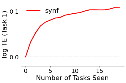
Plotting backward transfer efficiency
Backward transfer efficiency (BTE) measures the relative effect of future task data on the performance on a certain task.
It is the expected ratio of two risk functions of the learned hypothesis, one with access to the data up to and including the last observation from task t, and the other with access to the entire data sequence. The codes below uses the experiment results to calculate the average BTE numbers and display their changes over tasks learned.
[5]:
from functions.random_class_functions import calculate_results

# obtain bte results
btes = calculate_results(df_results, slot_num, shift_num)

# calculate the average numbers
bte = np.mean(btes, axis=0)

# setting plot parameters
fontsize = 22
ticksize = 20
[6]:
from functions.random_class_functions import plot_bte

plot_bte(bte, fontsize, ticksize)