Spoken Digit Experiment

---

This experiment will use an audio dataset named spoken_digit to test the performance of synergistic learning on audio classification tasks. The dataset consists of 3,000 recordings of digit (from 0 to 9) pronounced in English, by 6 speakers:

6 (speakers) x 10 (digits) x 50 (repetitions) = 3,000 (audio files)

Think MNIST for audio.

Import necessary packages and modules

import numpy as np
import IPython.display as ipd
from joblib import Parallel, delayed

Load spoken_digit data and extract features

To try on the up-to-date version of spoken_digit, we download the dataset from github repo (https://github.com/Jakobovski/free-spoken-digit-dataset) to our local disk. Find and copy the path of recordings. Here, the path is D:/Python Exploration/free-spoken-digit-dataset/recordings/.

Then we use librosa to load audio file, and extract the STFT (Short-time Fourier transform) feature. Since each audio has different durations, the STFT spectrograms vary in width. For convenience, we regularize the STFT spectrograms all to 28 by 28 images, using function provided by opencv.

Please ensure that you havelibrosaandopencvinstalled to run this experiment.

---

After running the block below, you will get:

audio_data: List of audio data, each item contains audio samples of a single digit. length = 3000

x_spec_mini: Numpy array of STFT spectrograms that have been resized to 28 by 28 image. shape = (3000, 28, 28)

y_number: Numpy array of labels indicating which digit is spoken. shape = (3000,)

y_speaker: Numpy array of first letter of the speaker. shape = (3000,)

from functions.spoken_digit_functions import load_spoken_digit

path_recordings = "./recordings/"

audio_data, x_spec_mini, y_number, y_speaker = load_spoken_digit(path_recordings)

Inspect data

Before running synergistic learning, let’s take a look at our audio data and spectrograms.

First, let’s play some audio of the digits!

num = 2999  # choose from 0 to 2999

print(
    "This is number",
    y_number[num],
    "spoken by speaker",
    y_speaker[num].upper(),
    "\nDuration:",
    audio_data[num].shape[0],
    "samples in",
    audio_data[num].shape[0] / 8000,
    "seconds",
)
ipd.Audio(audio_data[num], rate=8000)

This is number 4 spoken by speaker Y
Duration: 3857 samples in 0.482125 seconds

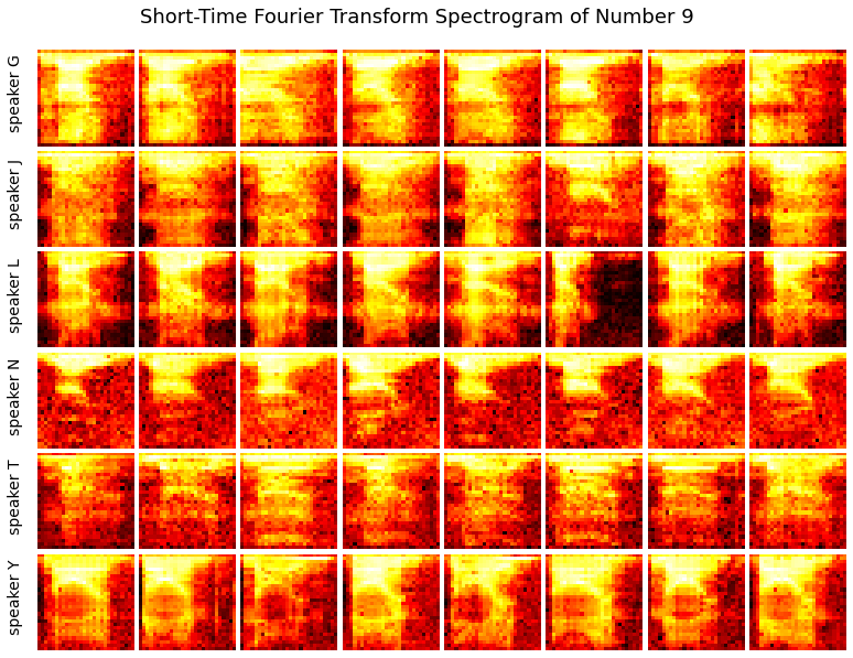
Now, let’s display STFT spectrograms of a same digit spoken by different speakers, and see if there is any distinguishable differences.

from functions.spoken_digit_functions import display_spectrogram

num = 9  # choose from 0 to 9
display_spectrogram(x_spec_mini, y_number, y_speaker, num)

Run Synergistic Learning

The Synergistic Learning project aims to improve program performance on sequentially learned tasks, proposing a lifelong learning approach.

It contains two different algorithms: Synergistic Forests (SynF) and Synergistic Network (SynN). SynF uses Uncertainy Forest as transformers, while SynN uses deep networks. These two algorithms achieve both forward knowledge transfer and backward knowledge transfer.

You can set model as ‘synf’ or ‘synn’ to choose which algorithm to use.

---

We divide tasks by speaker. As there are 6 speakers in total, we have 6 tasks.

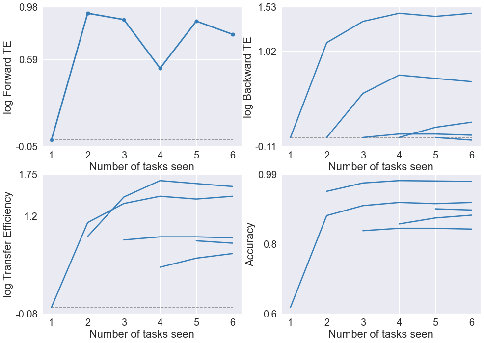
For each task at hand, we check whether the former tasks would forward-transfer knowledge to it, as well as whether the later tasks would backward-transfer knowledge to it, so that it has increased accuracy with more tasks seen.

Normally, we repeat the experiment for several times and average the results to get the expectation of generalization error. Choose num_repetition according to your computing power and time.

Prepare input data and start synergistic learning!

x = x_spec_mini.reshape(3000, 28, 28, 1)  # (3000,28,28,1)
y = y_number  # (3000,)
y_speaker = y_speaker  # (3000,), dtype: string

from functions.spoken_digit_functions import single_experiment

# Odin Model
model = "odin"
ntrees = 10  # number of trees, used when model is SynF
shuffle = False
num_repetition = 4  # fewer than actual figure to reduce running time

accuracy_list = Parallel(n_jobs=1)(
    delayed(single_experiment)(x, y, y_speaker, ntrees, model, shuffle)
    for _ in range(num_repetition)
)

accuracy_all_avg = np.average(accuracy_list, axis=0)

Calculate and plot transfer efficiency

• The transfer efficiency of algorithm \(f\) for given task \(t\) with sample size \(n\) is

  \[TE_n^t(f):=\mathbb{E}[R^t(f(D_n^{t}))]/\mathbb{E}[R^t(f(D_n))].\]

  We say that algorithm \(f\) has transfer learned for task \(t\) with data \(D_n\) if and only if \(TE_n^t(f)>1\).

• The forward transfer efficiency of \(f\) for task \(t\) given \(n\) samples is

  \[FTE_n^t(f):=\mathbb{E}[R^t(f(D_n^{t}))]/\mathbb{E}[R^t(f(D_n^{<t}))].\]

  We say an algorithm (positive) forward transfers for task \(t\) if and only if \(FTE_n^t(f)>1\).

• The backward transfer efficiency of \(f\) for task \(t\) given \(n\) samples is

  \[BTE_n^t(f):=\mathbb{E}[R^t(f(D_n^{<t}))]/\mathbb{E}[R^t(f(D_n))].\]

  We say an algorithm (positive) backward transfer for task \(t\) if and only if \(BTE_n^t(f)>1\).

For more details about FTE,BTE,TE and so on, please refer to the paper byVogelstein, et al. (2020)

from functions.spoken_digit_functions import calculate_results, plot_results

acc, bte, fte, te = calculate_results(accuracy_all_avg)
plot_results(acc, bte, fte, te, model)

Shuffled speaker

The default order of speakers is George followed by Jackson, Lucas, Nicolas, Theo, Yweweler. But we offer a variable shuffle. If we set shuffle = True, the order of speakers will be shuffled before each repetition starts.

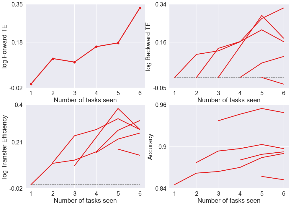
By shuffling the speakers and averaging the results, we can see the intrinsic trend of Synergistic Learning, i.e. the transfer efficiency increases monotonously with the ‘noises’ canceled out.

---

Here we use SynF for less computation cost, and set a reasonable number of repetitions.

model = "synf"
ntrees = 10  # number of trees
shuffle = True
num_repetition = 4  # fewer than actual figure to reduce running time

accuracy_list = Parallel(n_jobs=4)(
    delayed(single_experiment)(x, y, y_speaker, ntrees, model, shuffle)
    for _ in range(num_repetition)
)

accuracy_all_shuffle_avg = np.average(accuracy_list, axis=0)

acc, bte, fte, te = calculate_results(accuracy_all_shuffle_avg)
plot_results(acc, bte, fte, te, model)